Structured Model Use Cases
Use these guides after completing Build Your First Structured Model. Each starts with a modeling goal and ends with a result you can verify.
The guides share three mortgages so that the same records carry from one pattern to the next:
| loan | province | ltv | property_type | r |
|---|---|---|---|---|
| L-001 | ON | 0.82 | Detached | 0.15 |
| L-002 | BC | 0.82 | Condo | 0.15 |
| L-003 | SK | 0.82 | Multi-unit | 0.15 |
These are portfolio columns. r is the asset correlation carried by each loan.
Scenario inputs arrive as factors and are named where they are used.
Apply a haircut by category
Goal
Recovery on a defaulted mortgage is worse in some provinces than others. Apply a province-specific discount to LTV before it reaches the model.
Prerequisites
- dictionary columns named
ltvandprovince - an
adjusted_ltvpredictor or output queue column - familiarity with Local Transformations and Lookup References
Configure
Apply each discount in a Local Transformation, then have a Lookup Reference choose the transformation for the loan's province:
| Name | Kind | Definition |
|---|---|---|
ltv_on |
Local Transformation | {ltv} * 0.95 |
ltv_bc |
Local Transformation | {ltv} * 0.90 |
adjusted_ltv |
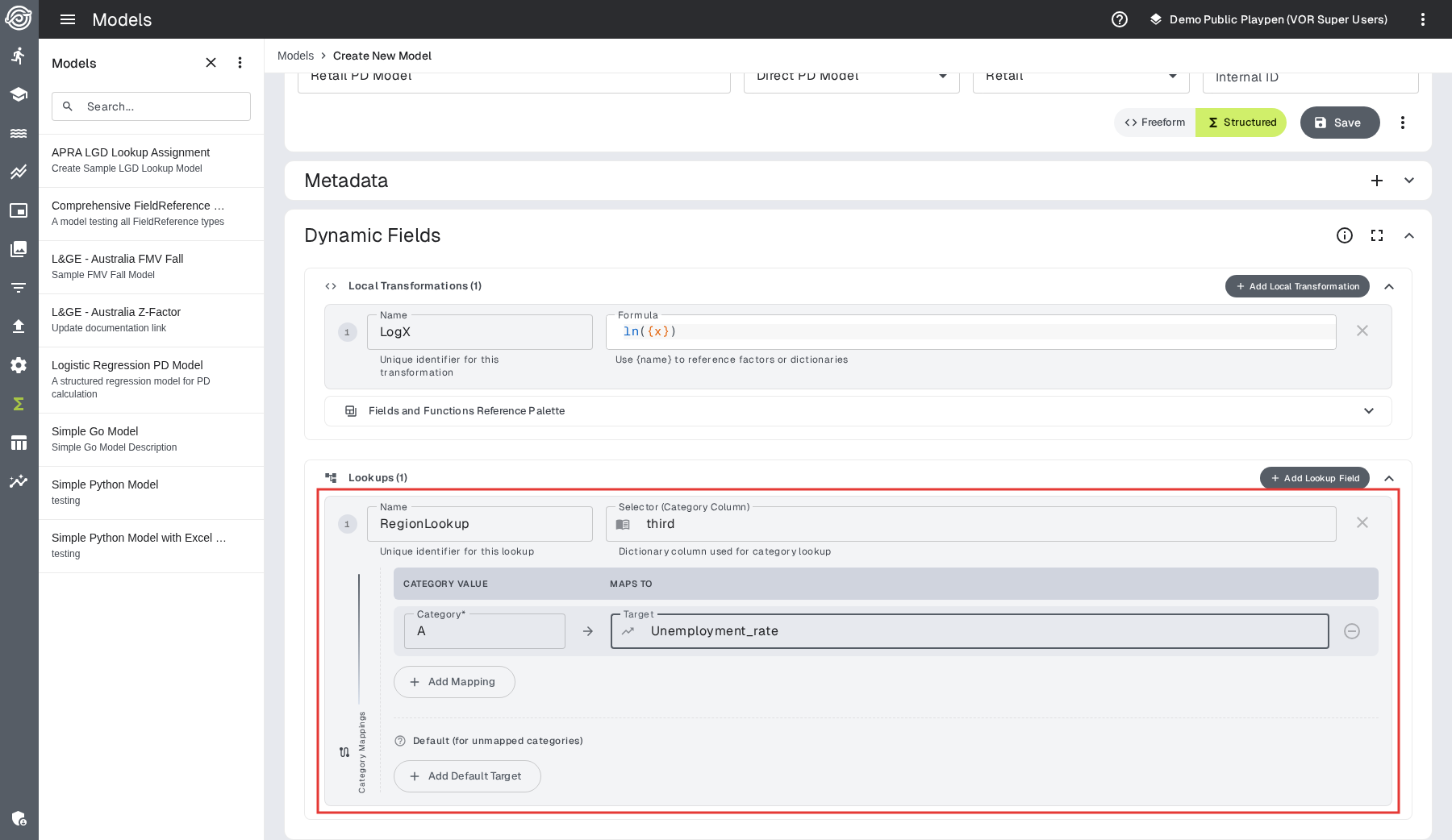
Lookup Reference | on {province}: ON → ltv_on, BC → ltv_bc, else dictionary ltv |
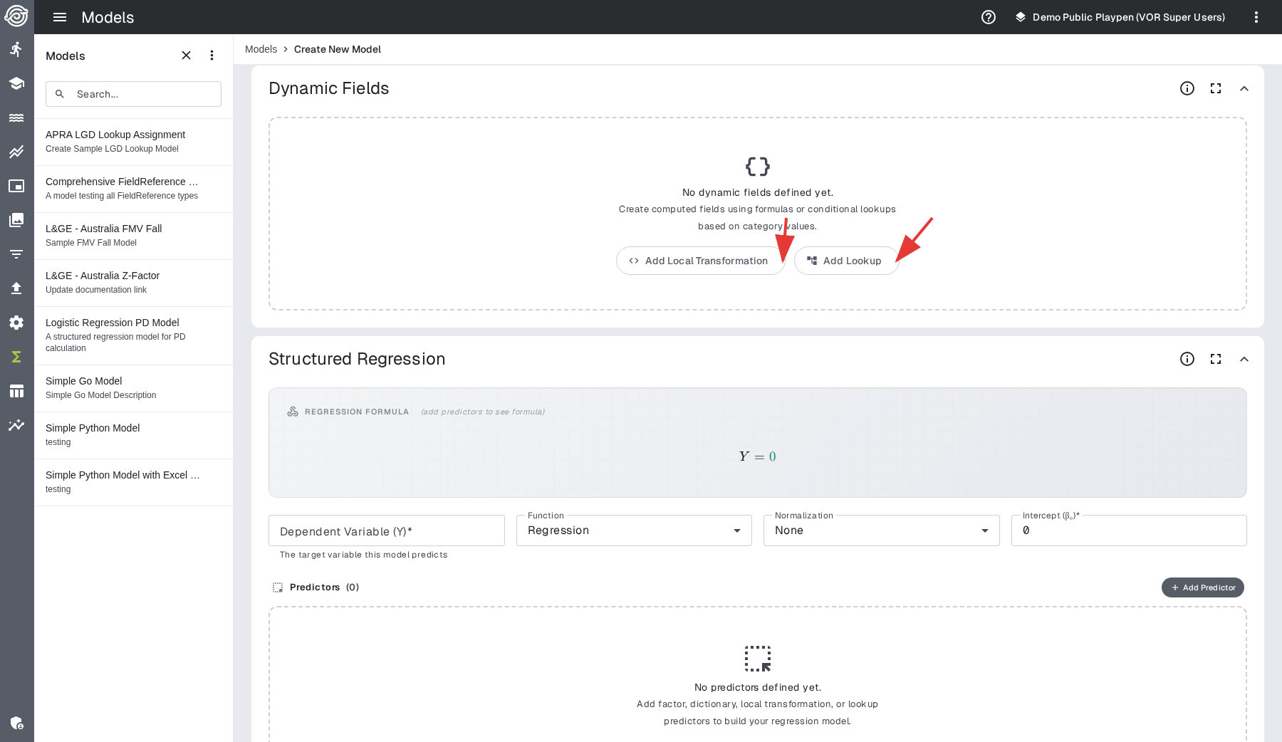
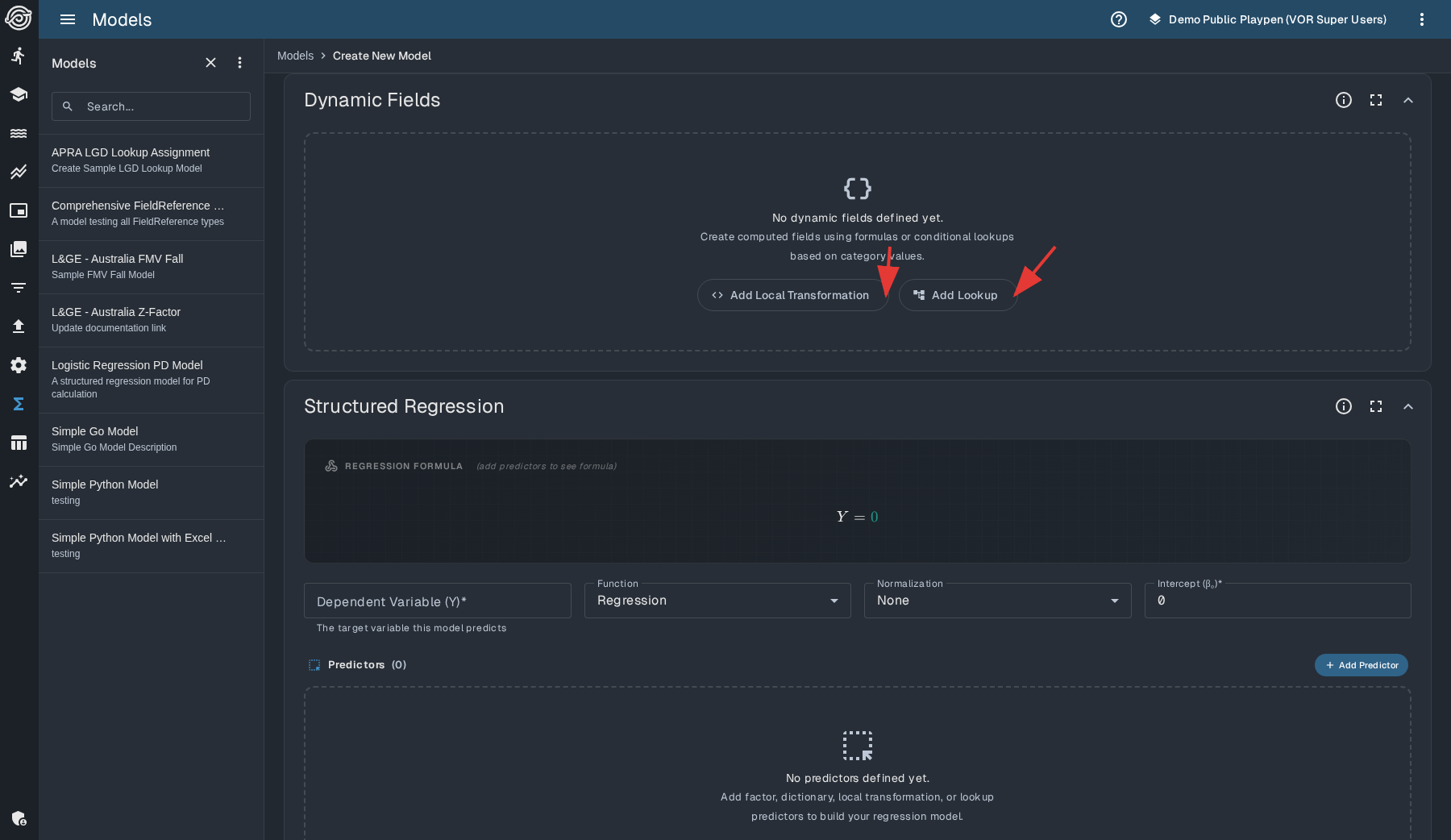
On the empty panel, use Add Local Transformation for ltv_on and ltv_bc:
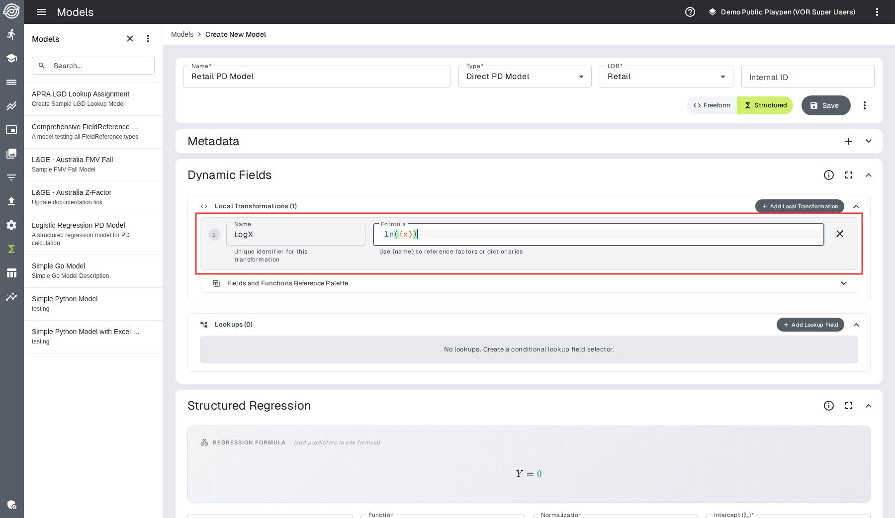
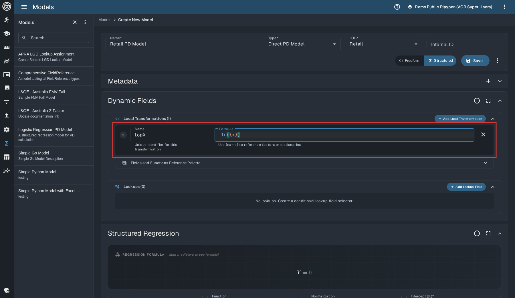
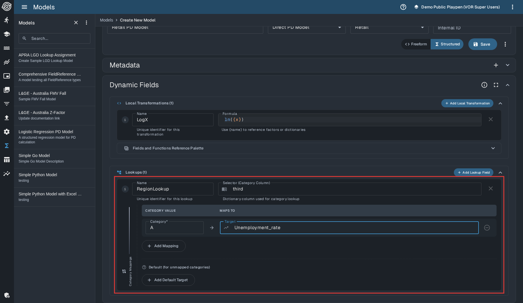
After adding the transformations, use Add Lookup Field in the Lookups section
for adjusted_ltv:
Reference adjusted_ltv as a predictor.
flowchart LR
    LTV[ltv] --> ON[ltv_on: ltv × 0.95]
    LTV --> BC[ltv_bc: ltv × 0.90]
    LTV --> L[adjusted_ltv lookup]
    ON --> L
    BC --> L
    P[province] --> L
    L --> R[predictor]
Expected result
Worked path: L-002
province = BC selects ltv_bc:
ltv = 0.82 → ltv_bc = 0.82 × 0.90 = 0.738 →
adjusted_ltv = 0.738 → predictor
| loan | province | ltv | target selected | adjusted_ltv |
|---|---|---|---|---|
| L-001 | ON | 0.82 | ltv_on |
0.779 |
| L-002 | BC | 0.82 | ltv_bc |
0.738 |
| L-003 | SK | 0.82 | ltv (default) |
0.820 |
Verify
Declare an output queue column named adjusted_ltv. The model writes the value
for every record beside the score, so the applied figure is visible without a
downstream SQL node. The example below names that model output queue
auditQueue; substitute your queue's name if it differs. Gate the audit file so
ordinary runs skip it:
out auditQueue -> audit.csv exec_when = audit
Set the flag in the Options tab of the Run Studies screen, in joboptions.json,
or with --exec-when. See
what a model node writes
and exec_when in Input / Output Nodes.
What you learned
- A lookup may target a Local Transformation, so the transformations compute the discounted values and the lookup only chooses between them.
- The engine evaluates transformations before lookups, independent of their position in the Dynamic Fields panel.
- A default target makes the Saskatchewan record fall through to the original
ltv; omitting the default makes an uncovered category fail the run.
Troubleshooting
Do not put the discounts in a haircut lookup and then calculate
{ltv} * {haircut} in a Local Transformation. The engine evaluates every
expression before resolving lookups, so that inverse dependency fails with
the input variable "haircut" to expression ... was not supplied. The formula
editor blocks it earlier with Unknown field: haircut.
Select a regional factor by category
Goal
A national house price index understates the exposure of a portfolio concentrated in one province. Make each loan follow its own regional series.
Prerequisites
- a
provincedictionary column - Ontario HPI, BC HPI and National HPI factors in the run's scenario
- a
regional_hpipredictor or output queue column
Configure
Create one Lookup Reference with factors as its targets:
| Name | Kind | Definition |
|---|---|---|
regional_hpi |
Lookup Reference | on {province}: ON → Ontario HPI, BC → BC HPI, else National HPI |
Reference regional_hpi directly as a predictor. It already yields the number
the predictor needs.
Expected result
Each record keeps its province and selects that province's scenario value at each horizon:
| loan | province | factor used | horizon 1 | horizon 2 | horizon 3 |
|---|---|---|---|---|---|
| L-001 | ON | Ontario HPI | 1.02 | 1.05 | 1.03 |
| L-002 | BC | BC HPI | 0.98 | 0.96 | 0.99 |
| L-003 | SK | National HPI | 1.00 | 1.01 | 1.02 |
Verify
Declare regional_hpi on an output queue and inspect its value beside the
province and horizon. L-001 should follow Ontario HPI, L-002 should follow BC
HPI, and L-003 should follow the default National HPI.
What you learned
A factor target is re-read at every horizon. A dictionary target is fixed for the life of the record. That difference determines whether a lookup follows a scenario series or a portfolio value.
Score a categorical field
Goal
Property type carries risk that no numeric field captures. Convert each category to a numeric contribution that can enter the regression.
Prerequisites
- a
property_typedictionary column - a
type_scorepredictor or output queue column - the conditional operator
Configure
Every lookup mapping target is a factor, dictionary column or Local
Transformation—not a numeric constant. Represent the category-to-number table
with one conditional Local Transformation named type_score:
{property_type} == "Detached" ? 0.0 : ({property_type} == "Condo" ? 0.3 : ({property_type} == "Multi-unit" ? 0.5 : 0.4))
Reference type_score as a predictor. Give it a coefficient of 1 so the scores
enter the equation unscaled, or fold the scaling into the coefficient and keep
the scores as relative weights.
Expected result
| loan | property_type | type_score | contribution at coefficient 1 |
|---|---|---|---|
| L-001 | Detached | 0.0 | 0.0 |
| L-002 | Condo | 0.3 | 0.3 |
| L-003 | Multi-unit | 0.5 | 0.5 |
Verify
Declare type_score on an output queue and compare it with property_type.
Test at least one category outside the three named branches to verify that the
final branch produces the deliberately chosen score of 0.4.
What you learned
A Local Transformation converts categories to numbers. A Lookup Reference selects a field, not a constant, so it serves a different modeling goal.
Troubleshooting
Comparisons are exact, so the final branch also handles spelling variants.
Choose its value deliberately: 0.0 and 0.4 score the loan very differently.
Use a lookup with no default instead when an uncovered category should fail the
run.
Every conditional needs a final branch, and every branch in this numeric formula must be decimal. A single whole-number branch fails only for records that reach that branch.
Estimate a PD, then stress it
Advanced: chain two models
This guide assumes you can configure model nodes and output queues. Complete the first three guides before using it as a walkthrough.
Goal
Estimate a probability of default, then feed that result into a second model that applies a severe systematic shock.
Prerequisites
adjusted_ltvfrom Apply a haircut by category- an Unemployment factor in the scenario
- an asset-correlation dictionary column named
r pdon the first model's output queue andstressed_pdon the second model's output queue
Configure
Use two models so the first model's output becomes an input to the downstream model:
flowchart LR
    P[Portfolio: ltv, province, r] --> PD[PD model with adjusted_ltv lookup]
    U[Unemployment factor] --> PD
    PD --> Q[Output queue: pd, r]
    Q --> S[Stress model]
    S --> O[stressed_pd]
First model: estimate the PD
Save this model as Mortgage PD. The normalization method turns the linear combination into a probability, so there is nothing to compute in a formula:
| Setting | Value |
|---|---|
| Dependent Variable (Y) | pd |
| Function | Regression |
| Normalization | Probit |
| Intercept (β₀) | -4.00 |
| Predictor | Kind | Coefficient (β) |
|---|---|---|
adjusted_ltv |
Lookup Reference | 1.40 |
| Unemployment | Factor | 0.08 |
This model reads a factor, so its node runs with scenario=true and emits one
record per loan per horizon. Declare a pd output column so the result is not
dropped.
Second model: stress the PD
Save this model as PD Stress and chain it after the first model. pd now
arrives as an ordinary input column. Create a Local Transformation named
stressed:
probnorm((probit({pd}) + sqrt({r}) * probit(0.999)) / sqrt(1 - {r}))
Pass the transformation through the equation unchanged:
| Setting | Value |
|---|---|
| Dependent Variable (Y) | stressed_pd |
| Function | Regression |
| Normalization | None |
| Intercept (β₀) | 0.00 |
| Predictor | Kind | Coefficient (β) | Exp |
|---|---|---|---|
stressed |
Local Transformation | 1.00 | 1 |
This model reads no factors, so its node does not need scenario=true. It runs
once per record of the queue it receives instead of expanding that queue over
the scenario a second time. Declare a stressed_pd output column.
Wire the model nodes
Ensure the output variables exist in src/dictionary.csv. The stressed row is
optional and supports the audit step at the end of this use case:
name,type,descr,arraylen,group,genformat
pd,num,Point-in-time probability of default,0,model_output,
adjusted_ltv,num,Category-adjusted LTV,0,model_output,
stressed_pd,num,Stressed probability of default,0,model_output,
stressed,num,Stress probability (model normalization None),0,model_output,
If the file already has a header, its column order may differ. Add only missing
variables, placing each value under the matching header. Existing rows must have
type num; keep their other metadata. If a name already has another type, use a
different name consistently in dictionary.csv, tables.csv, the model
settings, the process definition and the verification steps.
If portfolio already contains the other prerequisite columns, add the output
queues using the layout already present in src/tables.csv:
pd_output,,,PD model results,,portfolio,
pd_output,pd,num,Point-in-time probability of default,,,
pd_output,adjusted_ltv,num,Category-adjusted LTV,,,
stress_output,,,Stress model results,,pd_output,
stress_output,stressed_pd,num,Stressed probability of default,,,
stress_output,stressed,num,Stress probability (model normalization None),,,
pd_output,,PD model results,portfolio,
pd
adjusted_ltv
stress_output,,Stress model results,pd_output,
stressed_pd
stressed
The stressed field is optional. Do not mix the two layouts. The name layout
requires name as its first header because the parser recognizes each field by
its single-column row. Insert each field directly below its table row and before
the next table. The tablename,varname layout supports other header orders;
place each value under the matching header. Add only missing definitions, and
confirm pd_output inherits portfolio, stress_output inherits pd_output,
and every listed field resolves to type num. If an existing definition is
incompatible, use different names consistently throughout the dictionary,
tables, model settings, process and verification steps.
Then connect the two saved models in the process definition:
name structured_pd_stress

in input.csv -> portfolio

model (portfolio)(pd_output)
    model_name="Mortgage PD"
    scenario=true

model (pd_output)(stress_output)
    model_name="PD Stress"

out stress_output -> output.csv
Save the process as structured_pd_stress.strm, then register the added
variables before the tables and regenerate the queue and process code:
vor update dictionary --file src/dictionary.csv
vor update tables --file src/tables.csv
vor create queue --data src/tables.csv
vor create process structured_pd_stress.strm
Only the first model expands the portfolio over the selected scenario. The
second model receives those expanded records through pd_output.
Expected result
At one horizon with unemployment at 6.5, the first model produces:
| loan | adjusted_ltv | linear combination | pd |
|---|---|---|---|
| L-001 | 0.779 | -2.389 | 0.0084 |
| L-002 | 0.738 | -2.447 | 0.0072 |
| L-003 | 0.820 | -2.332 | 0.0099 |
With r = 0.15, the second model produces:
| loan | pd | stressed_pd |
|---|---|---|
| L-001 | 0.0084 | 0.0979 |
| L-002 | 0.0072 | 0.0876 |
| L-003 | 0.0099 | 0.1091 |
The displayed pd values are rounded; the second model receives the unrounded
values carried by the queue.
Verify
Inspect the queue between the two model nodes and the final output queue:
- Model 1 should write one
pdfor each loan and horizon. - The intermediate queue should carry both
pdandrto Model 2. - Model 2 should write one
stressed_pdfor each record it receives, without adding another set of scenario horizons.
Worked path: L-002
- Model 1:
-2.447→ Probit →pd = 0.0072 - Output queue:
pd = 0.0072 - Model 2:
pd = 0.0072,r = 0.15→ stress formula →stressed_pd = 0.0876
Declare stressed as an output queue column as well when you want to audit the
Local Transformation directly.
What you learned
- A model cannot read its own output, but a downstream model can read that value as an ordinary input column.
- Probit normalization turns the first model's linear combination into a PD.
- The stress formula converts the through-the-cycle PD into a normal-space threshold, adds a systematic shock scaled by the square root of the asset correlation, and converts the result back into a probability. A default rate under 1% becomes roughly 10% once the shock is applied.
Troubleshooting
If a run succeeds but pd or stressed_pd is missing, check that each dependent
variable matches a declared output queue column. A dependent variable matching no
column is dropped silently.
If the second model emits more horizons than the first, remove scenario=true from its model node. The first model already expanded the records over the scenario.
Next steps
- Review the field-reference dependency rules.
- Look up operators and functions in the Formula Language.
- Review model-node output behavior before adding audit columns.